Important
Users with versions dating prior to June 12 2013 please update. A nasty bug that caused the statistical part of mapDamage to use half of the data for estimation of the damage parameters, sorry for the inconvenience.
Contents
Introduction
mapDamage2 is a computational framework written in Python and R, which tracks and quantifies DNA damage patterns among ancient DNA sequencing reads generated by Next-Generation Sequencing platforms.
mapDamage was developed at the Centre for GeoGenetics by the palaeomix Orlando Group.
Requirements
- Python (version >= 3.7)
- pysam (version >= 0.6) python package, an interface for reading/writing SAM/BAM files
- Cython package, only necessary if pysam needs to be built
- gsl GNU scientific library (GSL)
- R libraries:
Of note, the R libraries and the GSL library are only required for the statistical estimation of DNA damage parameters. A stripped-down version of seqtk is included in this package for fast computation of reference base composition, it is written by Heng Li and can be found at here at github.
Installation
mapDamage2 was successfully tested on GNU/Linux and MacOSX environments.
Regular installation using pip
pip install mapdamageNews in version 2.0
- The main new feature is the approximate bayesian estimation of damage parameters.
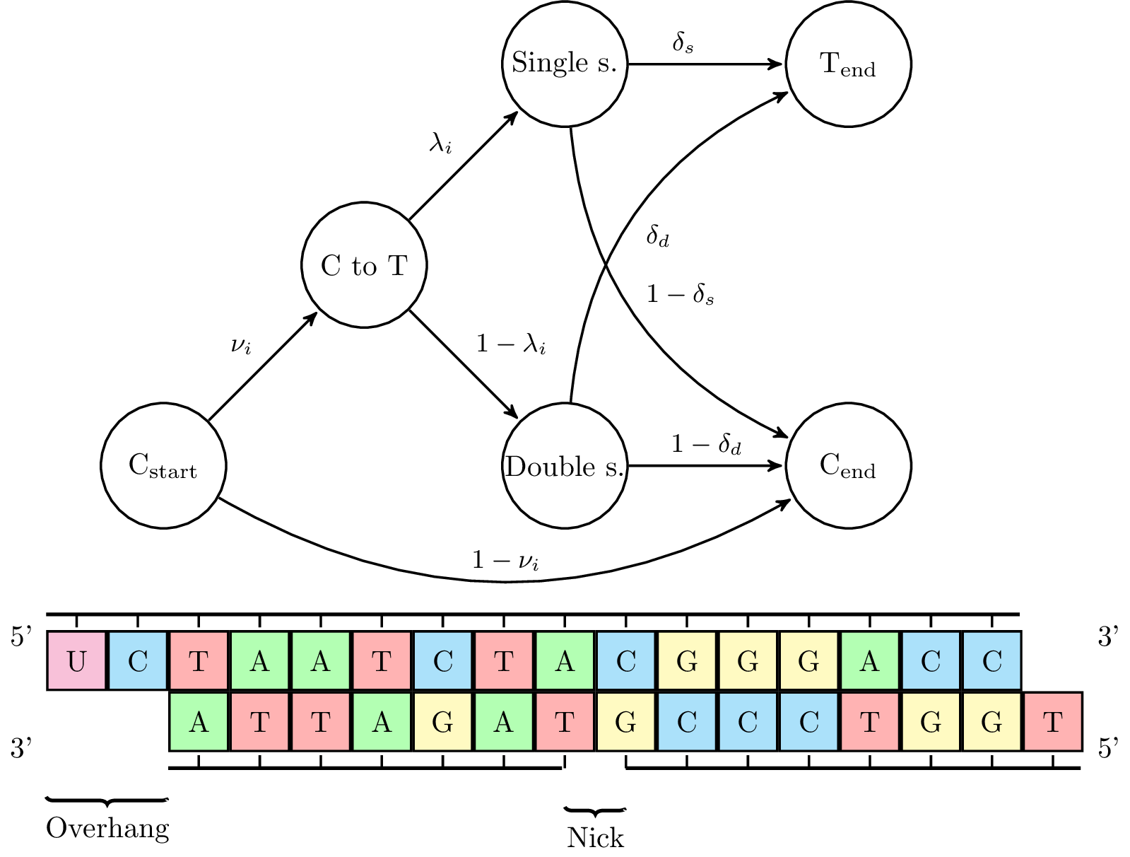
The idea behind the summary approach in mapdamage 2.0 is depicted in this figure:
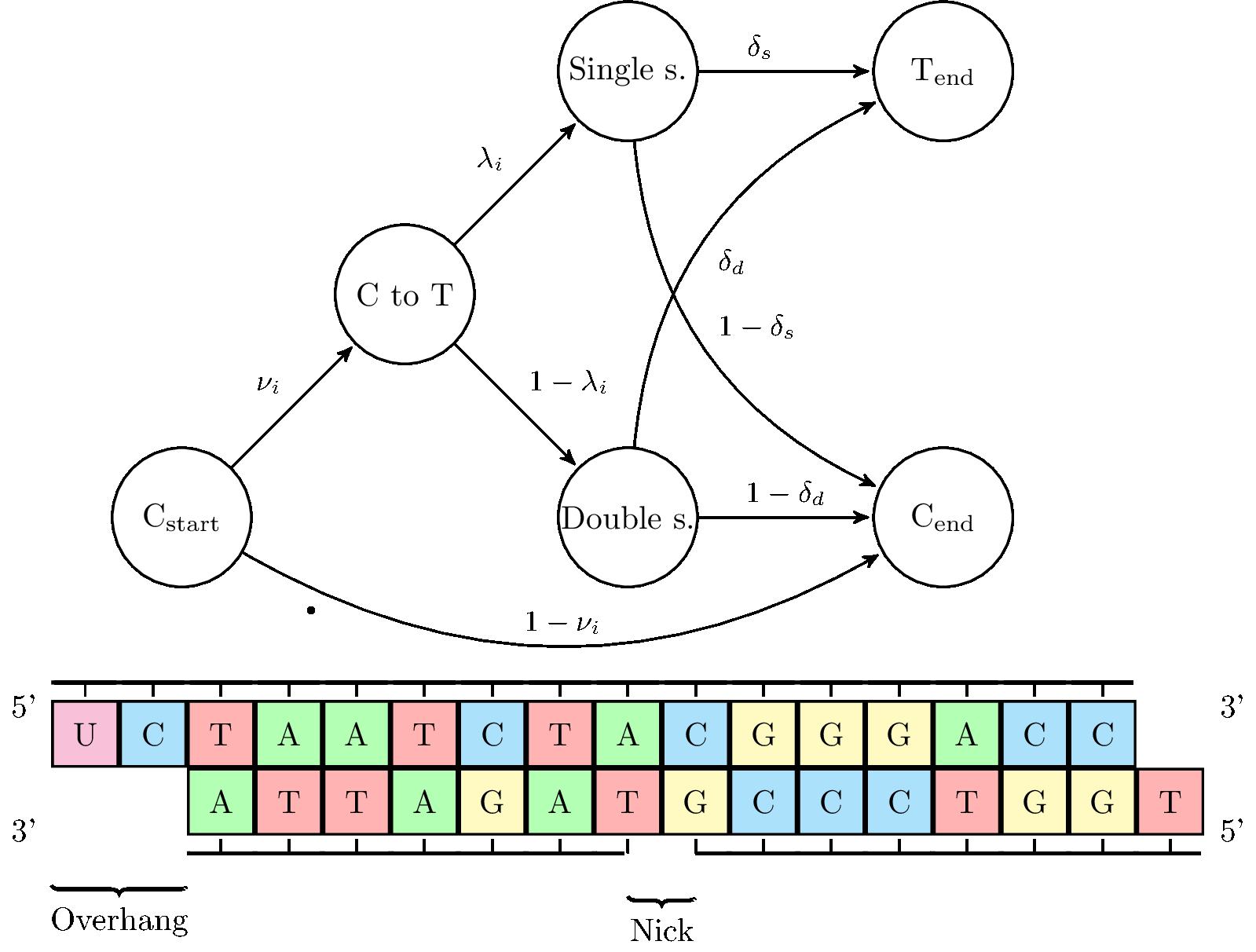
- The following four key damage parameters are estimated in Bayesian manner:
- Lambda, the probability of termating an overhang.
- DeltaD, the cytosine deamination probability in double strand context.
- DeltaS, the cytosine deamination probability in single strand context.
- Theta, the mean difference rate between the reference and the sequenced sample not due to DNA damage.
- The
--rescaleparameter can be optionally used to rescale quality scores of likely damaged positions in the reads. A new BAM file is constructed by downscaling quality values for misincorporations likely due to ancient DNA damage according to their initial qualities, position in reads and damage patterns. - The program was rewritten in python to make it simpler and the dependency on bedtools was replaced by the use of pysam. The memory footprint is now negligible and runtime reduced by ca. 25%.
- It is now possible to filter out nucleotides with qualities inferior to a threshold defined by users, allowing users to reduce the impact of sequencing errors when counting misincorporations.
Inputs
Two files are needed:
- A valid SAM/BAM file with a correct header, as argument to the
-ioption. - A FASTA file that contains reference sequences used for mapping reads, as argument to the
-roption.
References described in the SAM/BAM header and the FASTA file must be coherent, i.e, the references must have identical names and lengths. Extra sequences present in the FASTA header raise a warning but the program will proceed since all necessary references are available.
As an alternative, one can run only the plotting, statistic estimations or rescaling
on an already processed dataset. Use a combination of -d option followed by
a valid folder and the --plot-only, --stats-only or --rescale-only options.
Paired ends
We assume the pairs are facing inwards when counting the position specific misincorporations and rescaling quality scores. An additional assumption in the rescaling process is the pairs are non-overlapping. Make sure the pairing information in the BAM/SAM file is correct as we rely on the paired end information provided by the file. We advise not using non-overlapping paired ends coming from highly degraded samples (small template lengths) as they are likely contamination.
Output files
When all options are activated, 16 files are produced in the result folder.
Runtime_log.txt, log file with a summary of command lines used and timestamps.
For the plotting:
Fragmisincorporation_plot.pdf, a pdf file that displays both fragmentation and misincorporation patterns.Length_plot.pdf, a pdf file that displays length distribution of singleton reads per strand and cumulative frequencies of C->T at 5'-end and G->A at 3'-end are also displayed per strand.
Important remark: paired-ended reads are not considered for this analysis since the plot displays the distribution of read lengths and not insert sizes of paired-ended reads. For this last purpose, one can use the dedicated Picard tool CollectInsertSizeMetrics.misincorporation.txt, contains a table with occurrences for each type of mutations and relative positions from the reads ends.5pCtoT_freq.txt, contains frequencies of Cytosine to Thymine mutations per position from the 5'-ends.3pGtoA_freq.txt, contains frequencies of Guanine to Adenine mutations per position from the 3'-ends.dnacomp.txt, contains a table of the reference genome base composition per position, inside reads and adjacent regions.lgdistribution.txt, contains a table with read length distributions per strand.
For the statistical estimation:
Stats_out_MCMC_hist.pdf, MCMC histogram for the damage parameters and log likelihood.Stats_out_MCMC_iter.csv, values for the damage parameters and log likelihood in each MCMC iteration.Stats_out_MCMC_trace.pdf, a MCMC trace plot for the damage parameters and log likelihood.Stats_out_MCMC_iter_summ_stat.csv, summary statistics for the damage parameters estimated posterior distributions.Stats_out_post_pred.pdf, empirical misincorporation frequency and posterior predictive intervals from the fitted model.Stats_out_MCMC_correct_prob.csv, position specific probability of a C->T and G->A misincorporation is due to damage.dnacomp_genome.txt, contains the global reference genome base composition (computed by seqtk).- Rescaled BAM file, where likely post-mortem damaged bases have downscaled quality scores.
Examples and datasets
A simple command line that would process the entire BAM file with plotting and statistic estimation is:
mapDamage -i mymap.bam -r myreference.fasta
To run the plotting part with a new scale to fit lower levels of DNA damages, 0.1 as y-limit instead of 0.3 by default:
mapDamage -d results_mydata -y 0.1 --plot-only
Running the rescaling of the quality scores taking into account the damage estimates:
mapDamage -i mymap.bam -r myreference --rescale
To run the statistical estimation using only the 5'-ends and with verbose output:
mapDamage -d results_mydata --forward --stats-only -v
For further examples and usage introduction see the supplementary material chapter in the mapDamage2.0 manuscript.
Usage
Usage: mapDamage [options] -i BAMfile -r reference.fasta


Use option -h or --help for help


Options:


   --version             show program's version number and exit

   -h, --help            show this help message and exit


Input files:


    -i FILENAME, --input=FILENAME

                         SAM/BAM file, must contain a valid header, use '-' for reading a BAM from stdin

    -r REF, --reference=REF

                        Reference file in FASTA format

General options:

    -n DOWNSAMPLE, --downsample=DOWNSAMPLE

                        Downsample to a randomly selected fraction of the reads (if 0 < DOWNSAMPLE < 1),

                        or a fixed number of randomly selected reads (if DOWNSAMPLE >= 1). By default,

                        no downsampling is performed.

--downsample-seed   Seed value to use for downsampling. See documentation for py module 'random' for default behavior.

    -l LENGTH, --length=LENGTH

                        read length, in nucleotides to consider [70]

    -a AROUND, --around=AROUND

                        nucleotides to retrieve before/after reads [10]

    -Q MINQUAL, --min-basequal=MINQUAL

                        minimun base quality Phred score considered, Phred-33 assumed [0]

    -d FOLDER, --folder=FOLDER

                    folder name to store results [results_FILENAME]

    -f, --fasta         Write alignments in a FASTA file

    --plot-only         Run only plotting from a valid result folder

    -q, --quiet         Disable any output to stdout

    -v, --verbose       Display progression information during parsing


Options for graphics:


    -y YMAX, --ymax=YMAX

                        graphical y-axis limit for nucleotide misincorporation frequencies [0.3]

    -m READPLOT, --readplot=READPLOT

                        read length, in nucleotides, considered for plotting nucleotide

                        misincorporations [25]

    -b REFPLOT, --refplot=REFPLOT

                        the number of reference nucleotides to consider for ploting base

                        composition in the region located upstream and downstream of

                        every read [10]

    -t TITLE, --title=TITLE

                        title used for both graph and filename [plot]


Options for the statistical estimation:


    --rand=RAND         Number of random starting points for the likelihood optimization [30]

    --burn=BURN         Number of burnin iterations [10000]

    --adjust=ADJUST     Number of adjust proposal variance parameters iterations [10]

    --iter=ITER         Number of final MCMC iterations [50000]

    --forward=FORWARD   Using only the 5' end of the seqs [False]

    --reverse=REVERSE   Using only the 3' end of the seqs [False]

    --fix-disp=FIX_DISP Fix dispersion in the overhangs [True]

    --diff-hangs        The overhangs are different for 5' and 3'  [False]

    --fix-nicks=FIX_NICKS

                        Fix the nick frequency vector nu else estimate it with GAM [False]

    --jukes-cantor      Use Jukes Cantor instead of HKY85

    --single-stranded=SINGLE_STRANDED

                        Single stranded protocol [False]

    --seq-length=SEQ_LENGTH

                        How long sequence to use from each side [12]

    --stats-only        Run only statistical estimation from a valid result folder

    --rescale           Rescale the quality scores in the BAM file using the output from

                        the statistical estimation

    --rescale-only      Run only rescaling from a valid result folder

    --no-stats          Disabled statistical estimation, active by default
Description of tables
misincorporation table
This file looks like:
# table produced by mapDamage version 2.0

# using mapped file hits_sort_mts.bam and NC_012920.fasta as reference file

# Chr: reference from sam/bam header, End: from which termini of DNA sequences, Std: strand of reads

Chr End Std Pos A   C   G   T   Total   G>A C>T A>G T>C A>C A>T C>G C>A T>G T>A G>C G>T A>- T>- C>- G>- ->A ->T ->C ->G S

NC_012920.1 3p  +   1   424 579 201 424 1628    48  16  3   5   1   0   2   1   0   2   1   0   0   0   0   0   4   4   1   1   0

NC_012920.1 3p  +   2   466 535 213 404 1618    30  12  2   1   0   1   0   0   3   3   1   0   0   0   0   0   2   6   5   7   0

NC_012920.1 3p  +   3   514 463 223 417 1617    35  15  3   1   1   0   0   0   1   0   1   1   0   0   0   2   9   4   4   4   0

NC_012920.1 3p  +   4   514 483 221 400 1618    30  11  3   4   0   1   1   0   0   1   0   1   1   0   0   2   5   5   8   2   0
The first lines that start by a hash contain information about the options used while processing the data.
Then, the table contains occurrences of the 12 mutation type + 4 deletions + 4 insertions +
soft-clipping for each combination of reference (Chr column), strand (Std column) , end (End column) and position (Pos column).
In Z->X, Z comes from the reference, X is the nucleotide from reads. The columns A, C, G and T are the respective reference base count
and Total is the sum of the four reference nucleotides. Frequencies depicted in Fragmisincorporation_plot.pdf file are computed per
position as follows
#occurrences of mutations / #occurrences of the reference nucleotide
in order to compensate for reference base composition bias along the positions.
In this example, for G>A substitutions at the first base from the 3'-ends and for the positive strand:
48 / 201 = 0.238806
The Fragmisincorporation plot sums up misincorporations for all references and strand orientations, finally displays the frequencies per sequencing position.
5p means reads analyzed from their 5'-ends and are depicted at the bottom left.
3p means reads analyzed from their 3'-ends and are depicted at the bottom right.
Remark concerning soft-clipping:
Soft-clipped bases are bases located at read extremities that are NOT aligned to the reference. Those bases are not taken into account and alignments are computed on aligned bases. However, the soft-clipped bases are recorded and displayed as an orange line as a diagnostic for users. Even if, the positions for those bases are different from positions of all misincorporations, they should warn users that reads should be trimmed if soft-clipped base frequencies is high.
dnacomp table
Example table below:
# table produced by mapDamage version 2.0

# using mapped file hits_sort_mts.bam and NC_012920.fasta as reference file

# Chr: reference from sam/bam header, End: from which termini of DNA sequences, Std: strand of reads

Chr End Std Pos A   C   G   T   Total

NC_012920.1 3p  +   -70 113 77  43  181 414

NC_012920.1 3p  +   -69 178 140 97  233 648

NC_012920.1 3p  +   -68 230 145 98  219 692

NC_012920.1 3p  +   -67 217 157 76  272 722

NC_012920.1 3p  +   -66 224 188 88  239 739

NC_012920.1 3p  +   -65 244 165 104 262 775

NC_012920.1 3p  +   -64 223 185 102 288 798
The first lines that start by a hash contain information about the options used while processing the data.
Then, the table contains occurrences for each nucleotides, per reference (Chr column),
per strand (Std column) , per end (End column) and per position (Pos column).
At a given position, base composition is recorded either for the reference or for reads depending on the position and direction. The following table details which sequences and coordinates are used by default:
| Positions | 5p | 3p |
|---|---|---|
| negative values | reference, -10 to -1 | reads, -25 to -1 |
| positive values | reads, +1 to +25 | reference, +1 to +10 |
Stats_out_MCMC_iter_summ_stat table
This table contains the MCMC output of the five model parameters (depending on options) and log likelihood. The mean, standard deviation and quantiles per 2.5% interval
of the MCMC posterior simulations are reported. The
acceptance ratio (ratio of acceptances in the MCMC iterations) for each model parameter is calculated and depicted in the file and should be around 0.2. The companion file Stats_out_MCMC_iter.csv contains all the values obtained for each MCMC iteration and is available in graphical format as a histogram or a traceplot.
Example table below (the file is actually comma separated, here depicted with tabulations for clarity purposes):
	Theta			DeltaD			DeltaS			Lambda			Rho			LogLik

Mean	0.0129715432214025	0.0276128283764782	0.506870702430984	0.236778993065734	0.0429440323801133	-290.436006736216

Std.	0.000727998242592221	0.0016991302193519	0.0186911963483404	0.0112842920128649	0.0061180619558739	1.59627579978557

Acceptance ratio	0.1659	0.28692			0.17708			0.17222			0.21354			0.6781

0%	0.010343780887111	0.0200009808935262	0.443618434348717	0.196608727957609	0.024062021508867	-303.394224826161

2.5%	0.0115779148051722	0.0242216196897948	0.471593745448078	0.215033292540976	0.0316283681609979	-294.415675536748

5%	0.0117929060844704	0.0247964028136441	0.476538261177338	0.218032838581406	0.0334894928201135	-293.50800575224

7.5%	0.0119301611221827	0.0251693761425478	0.480224681410536	0.220351157627141	0.0345977332183658	-292.980765571483

10%	0.0120425513929948	0.0254336747705529	0.48309367716994	0.222245004085287	0.0354838414161916	-292.586815783461

12.5%	0.0121442465603967	0.0256581391709088	0.485339023472775	0.223852846490496	0.0361775294966489	-292.277395952081

15%...

.....
Stats_out_MCMC_correct_prob table
This table contains the position-specific probability of observing a C->T or a G->A due to a post-mortem damage.
Example table below (the file is actually comma separated, here depicted with tabulations for clarity purposes):
Position	C.T			G.A

1	1	0.980784246710695	0.65527195218869

2	2	0.97568346676245	0.71352845563181

3	3	0.969521194936301	0.743638120957285

4	4	0.962170583850572	0.766805824762406

5	5	0.953542075730188	0.787010580221663

6	6	0.943631337701685	0.803957830256353

7	7	0.932671721032529	0.81529717262592

8	8	0.921048902653476	0.82189320180069

9	9	0.909252012734666	0.825047159166101

10...

.....
Graphical outputs
Visualizing damage patterns
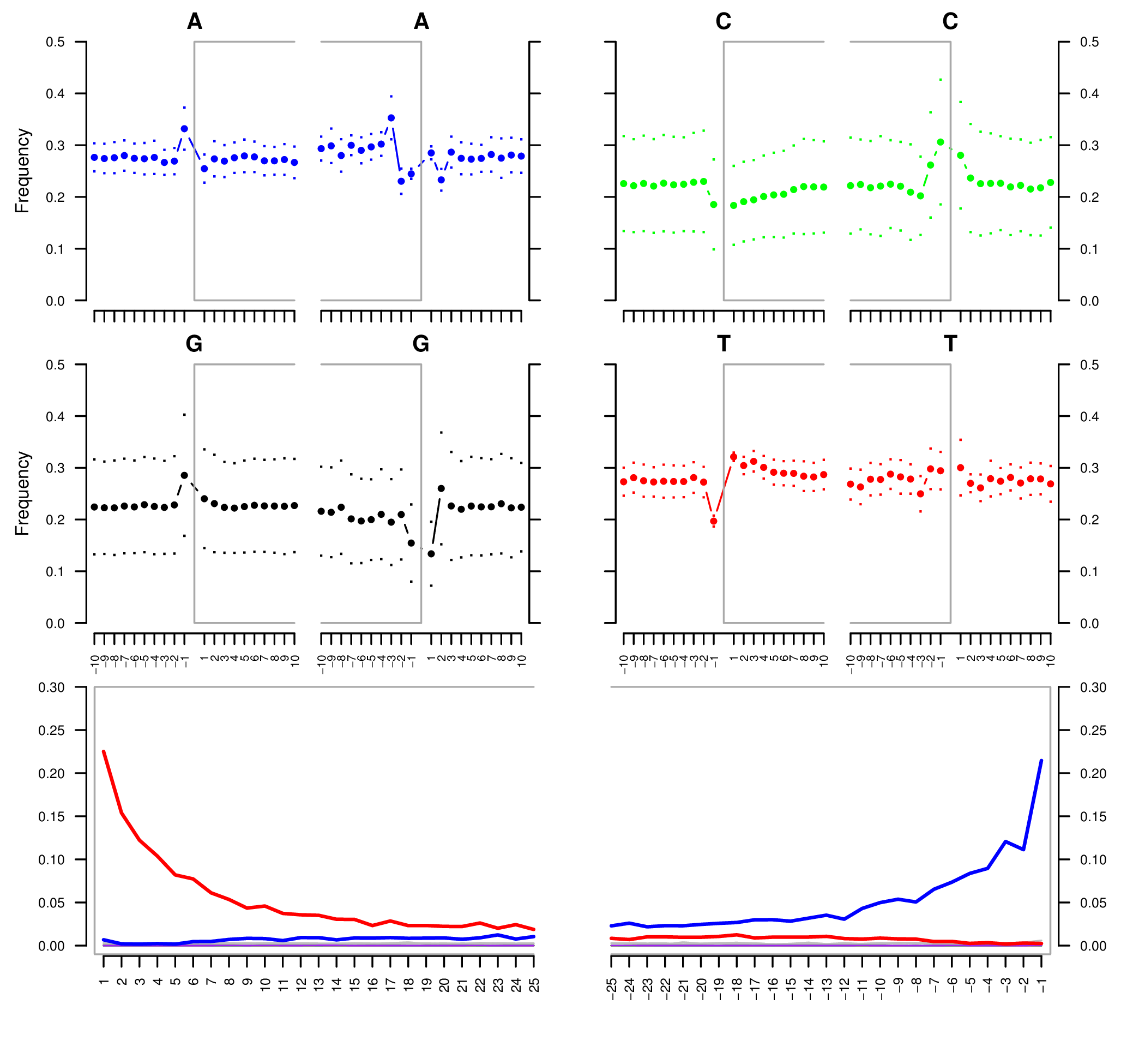
Sample E522. The four upper mini-plots show the base frequency outside and in the read (the open grey box corresponds to the read). The bottom plots are the positions' specific substitutions from the 5" (left) and the 3" end (right). The following color codes are used in the bottom plots:
- Red: C to T substitutions.
- Blue: G to A substitutions.
- Grey: All other substitutions.
- Orange: Soft-clipped bases.
- Green: Deletions relative to the reference.
- Purple: Insertions relative to the reference.
See Schuenemann et al. (2011) for more detailed information regarding the original data.
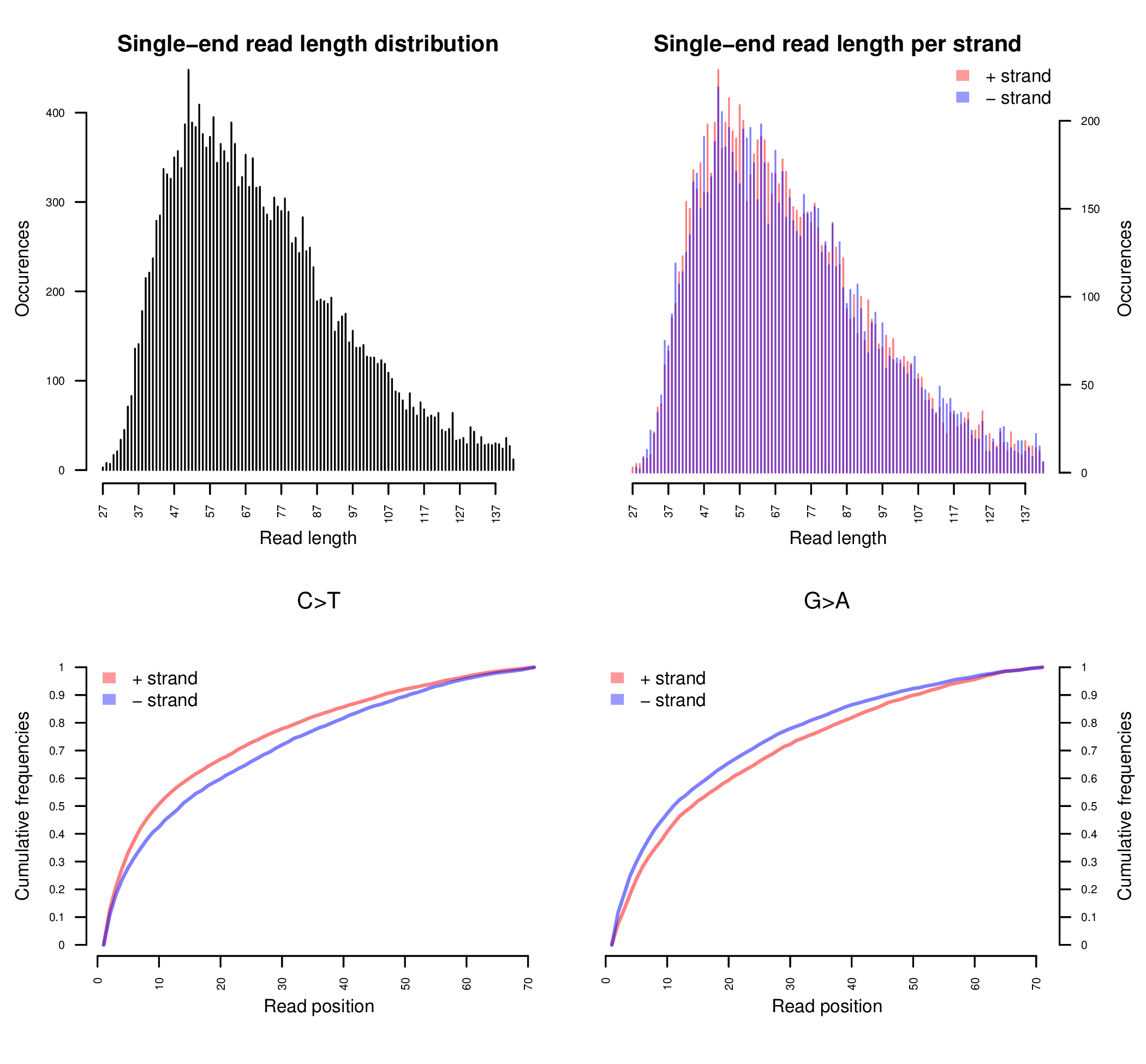
Sample E522. The upper two plots are histograms of the read lengths. The lower two plots are the empirical cumulative frequency of C->T and G->A misincorporations, normalized by the first 70 positions. See Schuenemann et al. (2011) for more detailed information regarding the original data.
Quantification of damage patterns

Sample E522.The empirical misincorporation frequencies and simulated posterior predictive intervals from the fitted model are depicted. See Schuenemann et al. (2011) for more detailed information regarding the original data.

Sample E522. Simulated posterior distributions of the five model parameters and log likelihood. See Schuenemann et al. (2011) for more detailed information regarding the original data.
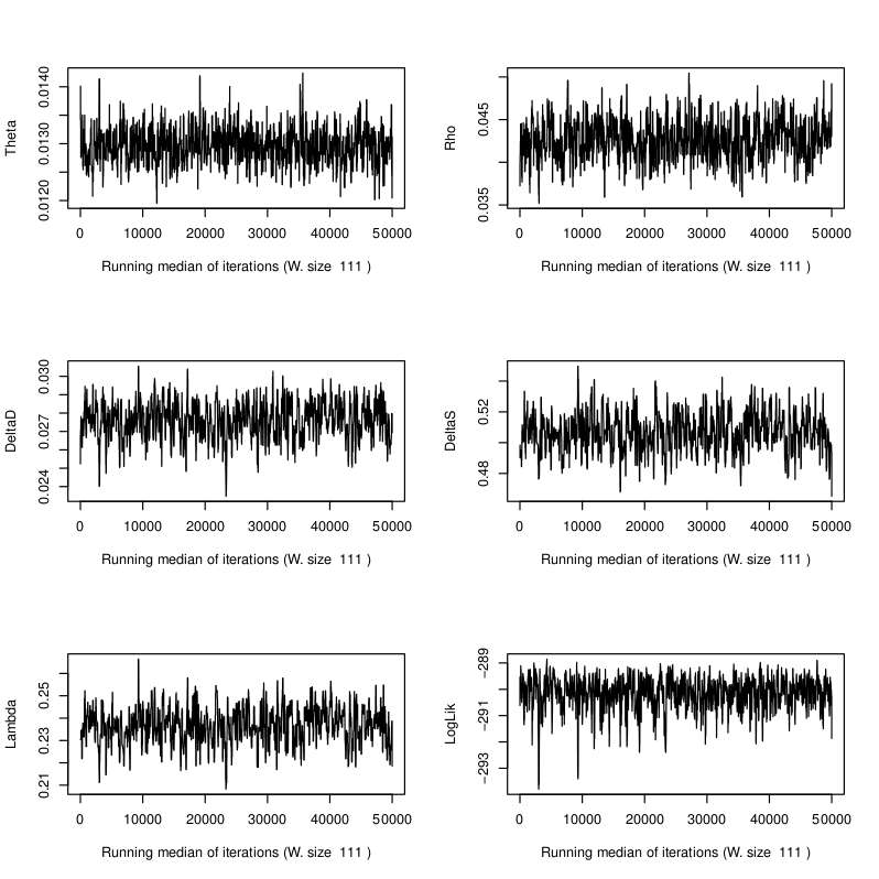
Sample E522. MCMC trace plots of the five model parameters and log likelihood. See Schuenemann et al. (2011) for more detailed information regarding the original data.
Citation
If you use this program, please cite the following publication:
Jónsson H, Ginolhac A, Schubert M, Johnson P, Orlando L.
mapDamage2.0: fast approximate Bayesian estimates of ancient DNA damage parameters.
Bioinformatics 2013. 23rd April 2013. doi: 10.1093/bioinformatics/btt193
The original mapDamage1 is described in the following article:
Ginolhac A, Rasmussen M, Gilbert MT, Willerslev E, Orlando L.
mapDamage: testing for damage patterns in ancient DNA sequences.
Bioinformatics 2011 27 (15):2153-2155
Schuenemann VJ, Bos K, DeWitte S, Schmedes S, Jamieson J, Mittnik A, Forrest S, Coombes BK, Wood JW, Earn DJ, White W, Krause J, Poinar HN. Targeted enrichment of ancient pathogens yielding the pPCP1 plasmid of Yersinia pestis from victims of the Black Death. Proc Natl Acad Sci USA. 2011 108:E746-52. doi: 10.1073/pnas.1105107108.
FAQ
Q: I got this error: could not find function "ggtitle"
A: update your ggplot2 package to at least version 0.9.2 by running:
update.packages("ggplot2")
and selecting a CRAN mirror
Q: How to clone the development version from github?
A: Use the following commands
git clone https://github.com/ginolhac/mapDamage.git
Contact
Please report bugs and suggest possible improvements on GitHub issues