Extract PDF tables to one tibble

From running times of the DEULUX 10k race
R
Author

Aurélien Ginolhac

Published

November 14, 2025

A German friend recently convinced me not only to start running but also to try a race.

He encouraged me to join the 10k DEULUX-Lauf which happens along the Sauer, half in Germany, half in Luxembourg, on November the 8th. This Race was the 33th organized in the small village of Langsur.

So far, not really any link to R. It comes.

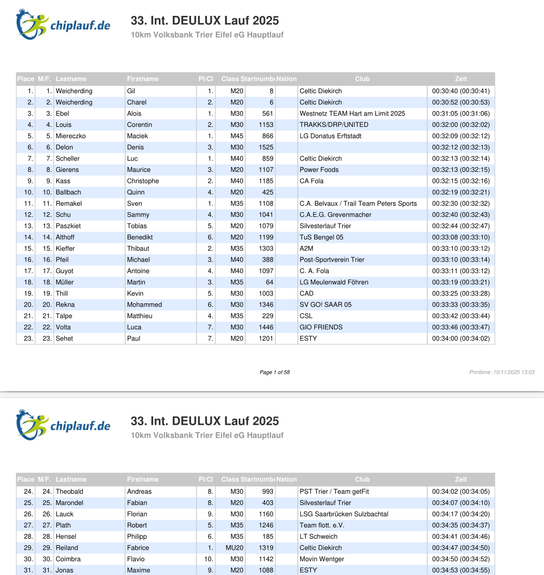
One can check his/her official time on the website chiplauf.de. The web-interface works well for querying the full results, by name, club, number but if you want all data, the only option is a PDF file.

It looks like this, 58 pages of tables:

Result PDF

PDF scrapping

I have never needed to so those things but it was in my radar. This was the occasion.

After a quick search, I ended up testing {tabulapdf} and this is excellent.

logo

See how you can the 58 pages tables in one tibble:

library(tidyverse)
library(tabulapdf)

fr <- "result list - 33. Int. DEULUX Lauf 2025 - 10km Volksbank Trier Eifel eG Hauptlauf.pdf"
seq_len(get_n_pages(fr)) |> 
   map_dfr(\(p) extract_tables(fr, pages = p)) -> zeit
zeit
# A tibble: 1,324 × 10
   Place `M/F.` Lastname    Firstname `Pl/Cl` `Class S` artnumb `Nr ation` Club 
   <dbl>  <dbl> <chr>       <chr>       <dbl> <chr>       <dbl> <lgl>      <chr>
 1     1      1 Weicherding Gil             1 M20             8 NA         Celt…
 2     2      2 Weicherding Charel          2 M20             6 NA         Celt…
 3     3      3 Ebel        Alois           1 M30           561 NA         West…
 4     4      4 Louis       Corentin        2 M30          1153 NA         TRAK…
 5     5      5 Miereczko   Maciek          1 M45           866 NA         LG D…
 6     6      6 Delon       Denis           3 M30          1525 NA         NA   
 7     7      7 Scheller    Luc             1 M40           859 NA         Celt…
 8     8      8 Gierens     Maurice         3 M20          1107 NA         Powe…
 9     9      9 Kass        Christop…       2 M40          1185 NA         CA F…
10    10     10 Ballbach    Quinn           4 M20           425 NA         NA   
# ℹ 1,314 more rows
# ℹ 1 more variable: Zeit <chr>
# ℹ Use `print(n = ...)` to see more rows

We are missing the country of origin, which was asked at registration. Another PDF of registered people is available:

reg <- "liste des participants - 33. Int. DEULUX Lauf 2025 - 10km Volksbank Trier Eifel eG Hauptlauf.pdf"
seq_len(get_n_pages(reg)) |> 
   map_dfr(\(p) extract_tables(reg, pages = p)) -> registrations
registrations
# A tibble: 1,560 × 5
   Nom     `Prénom`  `M/F`    Nation Club               
   <chr>   <chr>      <chr>    <chr>  <chr>              
 1 Sander  Cosima     féminin  NA     Team Slowmotion    
 2 Sander  Anna       féminin  NA     Team Slowmotion    
 3 Schmit  Mike       masculin NA     Spiridon Lëtzebuerg
 4 Quintus Nancy      féminin  NA     RBUAP              
 5 Clement Manuel     masculin NA     Die Eifelläufer    
 6 Ochs    Svenja     féminin  NA     NA                 
 7 Berg    Alwin      masculin NA     Die Eifelläufer    
 8 Lanter  Tom        masculin LUX    NA                 
 9 Weber   Christiane féminin  LUX    NA                 
10 Vesque  Yves       masculin LUX    CGDIS              
# ℹ 1,550 more rows
# ℹ Use `print(n = ...)` to see more rows

We see that 1560 people registered and 1324 actually ran the event.

But looking at the Nation column we were after, it is missing for most of the people so we don’t bother more with that

Code
count(registrations, Nation, sort = TRUE)
# A tibble: 27 × 2
   Nation     n
   <chr>  <int>
 1 <NA>    1323
 2 DEU      126
 3 LUX       60
 4 FRA        7
 5 Deutsc     6
 6 ITA        6
 7 Luxem      4
 8 USA        3
 9 BEL        2
10 COL        2
# ℹ 17 more rows

Let’s tidy things a bit with getting the time (as the right data type thanks to `{readr} helper!), age category and the sex of participants:

Code
zeit |> 
   mutate(sex = str_extract(`Class S`, "[MW]"),
          time = str_extract(Zeit, "\\d{2}:\\d{2}:\\d{2}") |> parse_time(),
          age = str_extract(`Class S`, "\\d+")) |> 
   select(Place, Firstname, age, dossard = artnumb, sex, class = `Class S`, Club, time) -> deulux
head(deulux, 10L) |> knitr::kable()
Place Firstname age dossard sex class Club time
1 Gil 20 8 M M20 Celtic Diekirch 00:30:40
2 Charel 20 6 M M20 Celtic Diekirch 00:30:52
3 Alois 30 561 M M30 Westnetz TEAM Hart am Limit 2025 00:31:05
4 Corentin 30 1153 M M30 TRAKKS/DRP/UNITED 00:32:00
5 Maciek 45 866 M M45 LG Donatus Erftstadt 00:32:09
6 Denis 30 1525 M M30 NA 00:32:12
7 Luc 40 859 M M40 Celtic Diekirch 00:32:13
8 Maurice 20 1107 M M20 Power Foods 00:32:13
9 Christophe 40 1185 M M40 CA Fola 00:32:15
10 Quinn 20 425 M M20 NA 00:32:19

Time densities

Let’s display the shape of the time densities and where I am located.

Code
deulux |> 
   ggplot(aes(x = time)) +
   geom_density() + 
   geom_vline(data = \(x) filter(x, dossard == 725), aes(xintercept = time),
              color = "steelblue", linetype = "dashed") +
   geom_text(data = \(x) filter(x, dossard == 725), aes(y = .00008, label = Firstname),
              color = "steelblue", nudge_x = 300) +
   labs(title = "All DEULUX participants",
        y = "Density") +
   theme_bw(14)

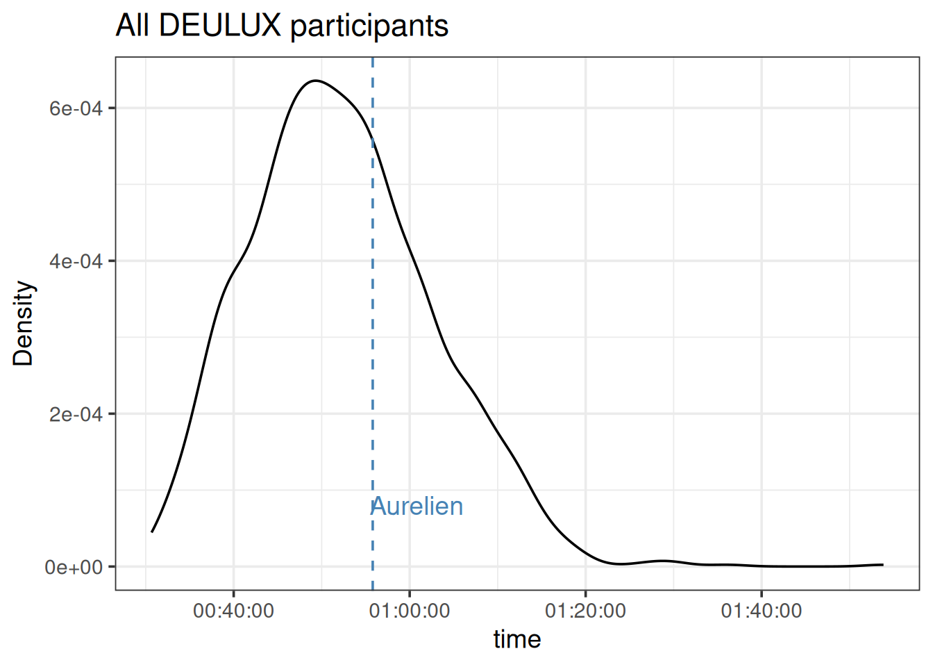
Most people aimed at 50 minutes, with a discrete but present shoulder for 40 minutes. Actually one pacer was participating for this time, showing the interest for this competitive time. After 80 minutes, most people crossed the the finnish line with a right-tail.
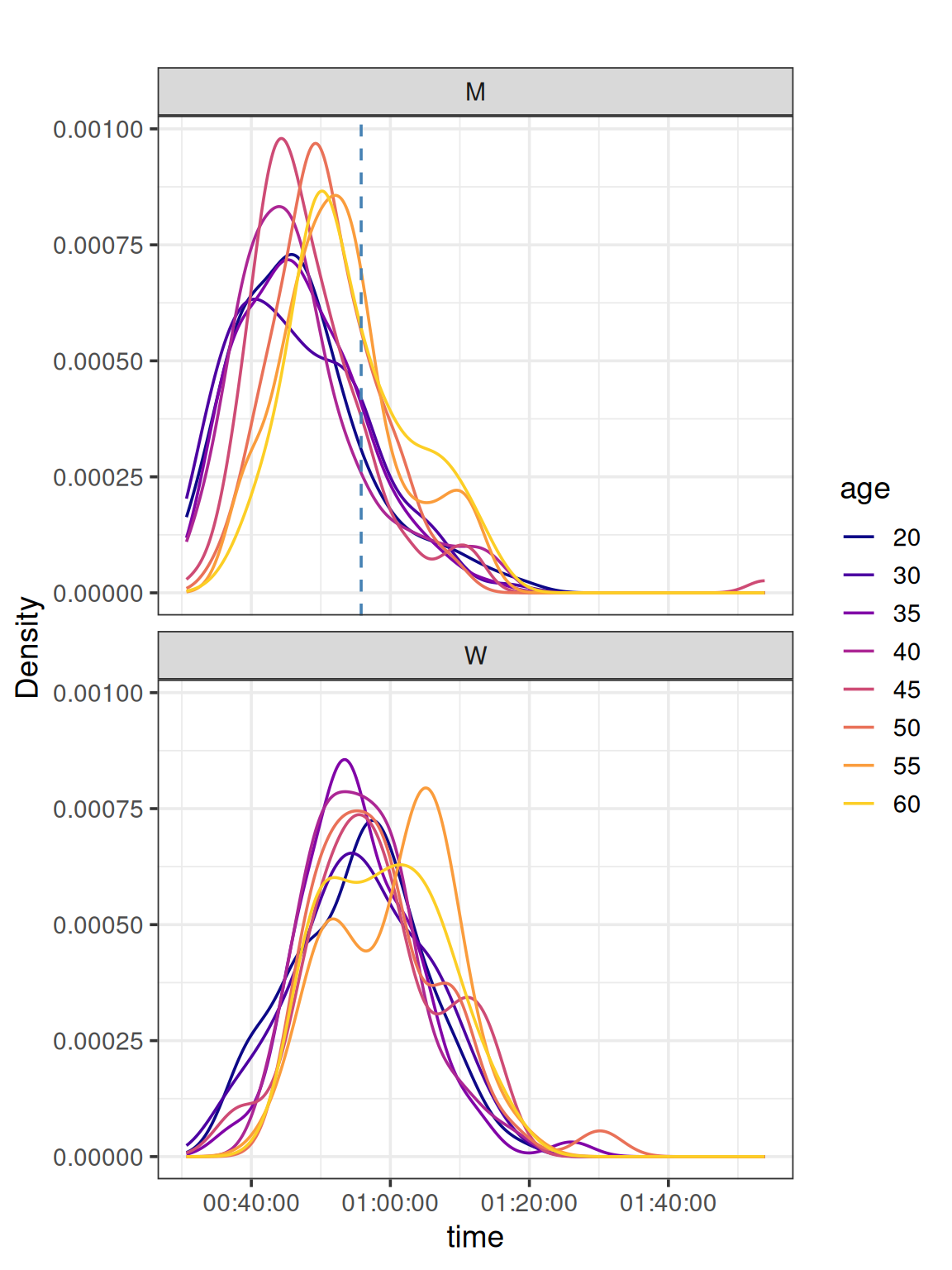
Code
deulux |> 
   mutate(quantile = cume_dist(time)) |> 
   filter(dossard == 725) |> 
   select(time:quantile)
# A tibble: 1 × 2
  time   quantile
  <time>    <dbl>
1 55'48"    0.655

Precisely, I was the 68.48 percentile.

Split by sex

Splitting by sex shows that I ended up like most women.

Code
deulux |> 
   ggplot(aes(x = time, colour = sex)) +
   geom_line(stat = "density") + 
   geom_vline(data = \(x) filter(x, dossard == 725), aes(xintercept = time),
              color = "steelblue", linetype = "dashed") +
   geom_text(data = \(x) filter(x, dossard == 725), aes(y = .00008, label = Firstname),
              color = "steelblue", nudge_x = 350) +
   scale_colour_manual(values = c("steelblue", "purple")) +
   labs(title = "All DEULUX participants",
        y = "Density") +
   theme_bw(14)

Split by age

First, let’s see how many participants are per age category

Code
ggplot(deulux, aes(x = age, fill = sex)) +
   geom_bar() +
   theme_bw() +
    scale_fill_manual(values = c("steelblue2", "purple"))

Code
deulux |> 
   filter(between(as.integer(age), 20, 60)) |> 
   ggplot(aes(x = time, colour = age)) +
   geom_line(stat = "density") + 
   geom_vline(data = \(x) filter(x, dossard == 725), aes(xintercept = time),
              color = "steelblue", linetype = "dashed") +
   # tweak the end to avoid the yellow we can't see much
   scale_colour_viridis_d(end = 0.9, option = "plasma") +
   facet_wrap(vars(sex), ncol = 1) +
   labs(title = "",
        y = "Density") +
   theme_bw(14)

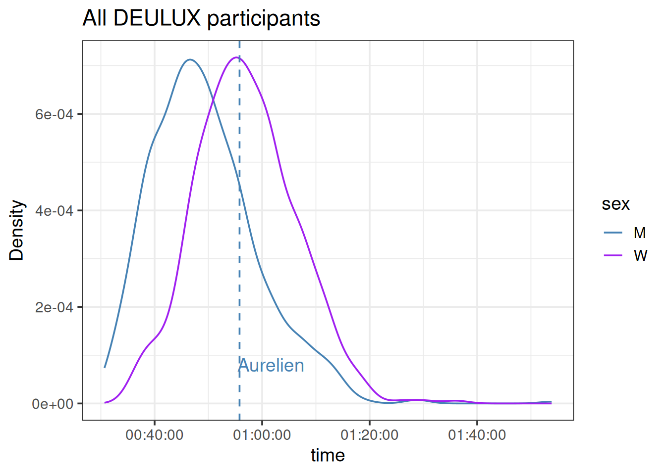
As expected, older people performed less than younger ones. But in details, 60+ men do better than 55+. Actually, we observe the same for women. For this category of 55+, the two sub-populations in men and women have opposite quantities. The faster 55+ women are a smaller group while most 55+ men are faster.

Belonging to a club

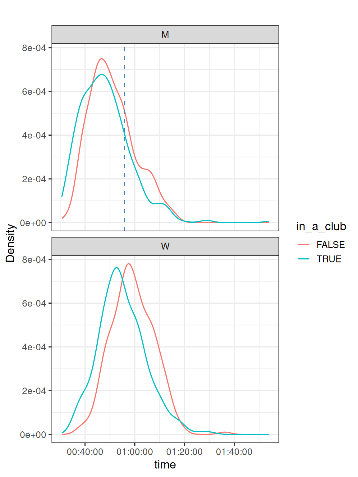
One could imagine that people running in a club are more trained. We can check this assumption for this race

Code
deulux |> 
   mutate(in_a_club = !is.na(Club)) |> 
   ggplot(aes(x = time, colour = in_a_club)) +
   geom_line(stat = "density") + 
   geom_vline(data = \(x) filter(x, dossard == 725), aes(xintercept = time),
              color = "steelblue", linetype = "dashed") +
   facet_wrap(vars(sex), ncol = 1) +
   labs(title = "",
        y = "Density") +
   theme_bw(14)

Interesting plot! For women, being in a club increase the performance in this race, shifting the densities to faster time. For men, the shape changes, faster time are more frequent for people club but the mode remain globally the same.
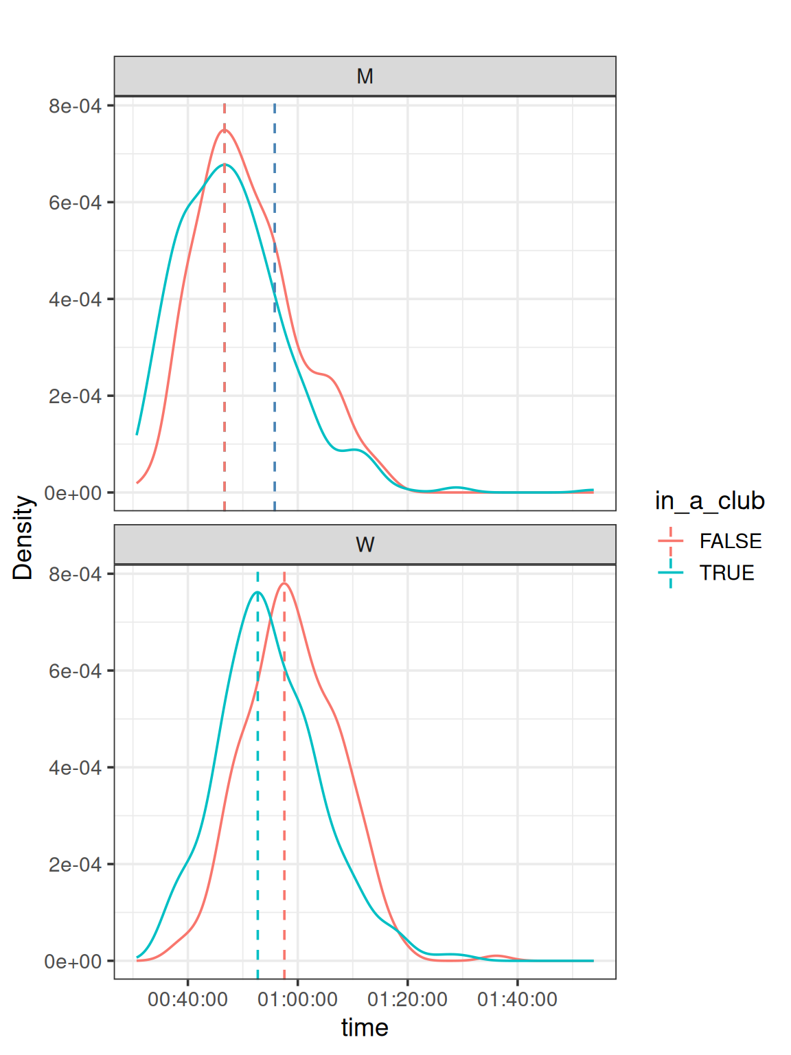
Conclusion

The {tabulapdf} package does a great job! Reports the number of pages and can neatly extract each table to a tibble. Was fun to plot densities of this race, will be curious to plot more as I have no idea how representative this race was compare to others.